Science Data Processing Workflow

General Workflow for Generating Association Products

See Associations and JWST for an overview of how JWST uses associations. This document describes how associations are used by the ground processing system to execute the stage 2 and stage 3 pipelines.

Up to the initial calibration step calwebb_detector1, the science exposures are treated individually. However, starting at the stage 2 calibration step, exposures may need other exposures in order to be further processed. Instead of creating a single monolithic pipeline, the workflow uses the associations to determine what pipeline should be executed and when to execute them. In the figure below, this wait-then-execute process is represented by the workflow trigger. The workflow reads the contents of an association file to determine what exposures, and possibly other files, are needed to continue processing. The workflow then waits until all exposures exist. At that point, the related calibration pipeline is executed with the association as input.

With this finer granularity, the workflow can run more processes parallel, and allows the operators deeper visibility into the progression of the data through the system.

Figure 1: General workflow through stage 2 and stage 3 processing

The figure represents the following workflow:

• Data comes down from the observatory and is converted to the raw FITS files.

• calwebb_detector1 is run on each file to convert the data to the countrate format.

• In parallel with calwebb_detector1, the Pool Maker collects the list of downloaded exposures and places them in the Association Pool.

• When enough exposures have been download to complete an Association Candidate, such as an Observation Candidate, the Pool Maker calls the Association Generator, asn_generate, to create the set of associations based on that Candidate.

• For each association generated, the workflow creates a file watch list from the association, then waits until all exposures needed by that association come into existence.

• When all exposures for an association exist, the workflow then executes the corresponding pipeline, passing the association as input.

Wide Field Slitless Spectroscopy

In most cases, the data will flow from stage 2 to stage 3, completing calibration. However, more complicated situations can be handled by the same wait-then-execute process. One particular case is for the Wide Field Slitless Spectrometry (WFSS) modes. The specific flow is show in the figure below:

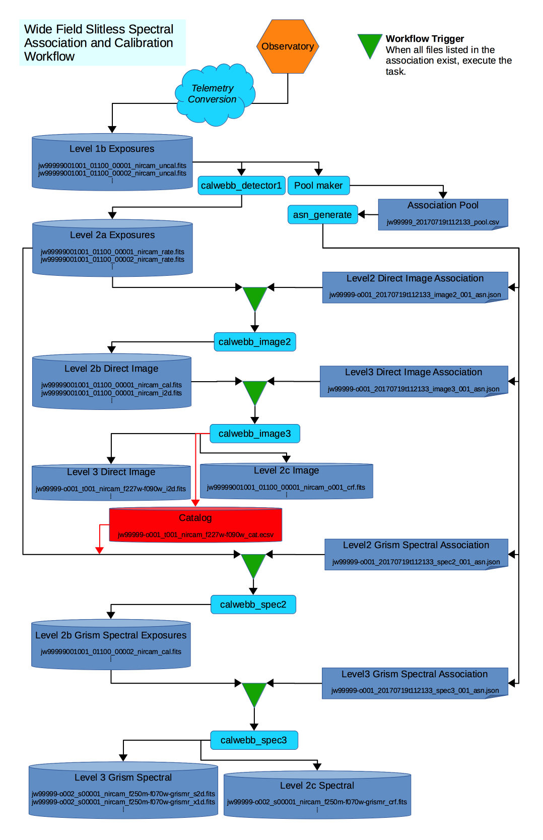
Figure 2: WFSS workflow

For WFSS data, at least two observations are made, one consisting of a direct image of the field-of-view (FOV), and a second where the FOV is dispersed using a grism. The direct image is first processed through stage 3. At the stage 3 stage, a source catalog of objects found in the image, and a segmentation map, used to record the minimum bounding box sizes for each object, are generated. The source catalog is then used as input to the stage 2 processing of the spectral data. This extra link between the two major stages is represented by the Segment & Catalog file set, shown in red in the diagram. The stage 2 association grism_spec2_asn not only lists the needed countrate exposures, but also the catalog file produced by the stage 3 image processing. Hence, the workflow knows to wait for this file before continuing the spectral processing.