Description
- Class:
- Alias:
photom
The photom step applies flux (photometric) calibrations to a data product
to convert the data from units of countrate to surface brightness (or, in
some cases described below, to units of flux density).
The calibration information is read from a
photometric reference file.
The exact nature of the calibration information loaded from the reference file
and applied to the science data depends on the instrument mode, as
described below.
This step relies on having wavelength information available when working on
spectroscopic data and therefore the
assign_wcs step must be applied before executing
the photom step. Pixels with wavelengths that are outside of the range
covered by the calibration reference data are set to zero and flagged
in the DQ array as “DO_NOT_USE.”
Some spectroscopic modes also rely on knowing whether the target is a point
or extended source and therefore the
srctype step must be applied before executing
the photom step.
Upon successful completion of this step, the status keyword S_PHOTOM will be set to “COMPLETE”. Furthermore, the BUNIT keyword value in the SCI and ERR extension headers of the science product are updated to reflect the change in units.
Imaging and non-IFU Spectroscopy
Photom Data
For these instrument modes the PHOTOM Reference File contains a table of
exposure parameters that define various instrument configurations and the flux
conversion data for each of those configurations. The table contains one row
for each allowed combination of exposure parameters,
such as detector, filter, pupil, and grating. The photom step searches the
table for the row that matches the parameters of the science exposure and
then loads the calibration information from that row of the table.
Note that for NIRSpec fixed-slit mode, the step will search the table
for each slit in use in the exposure, using the table row that corresponds to
each slit.
For these table-based PHOTOM reference files, the calibration information in each
row includes a scalar flux conversion constant, as well as optional arrays of
wavelength and relative response (as a function of wavelength).
For spectroscopic data, if the photom step finds that the wavelength and relative
response arrays in the reference table row are populated, it loads those 1-D arrays
and interpolates the response values into the 2-D space of the science image based
on the wavelength at each pixel.
For NIRSpec spectroscopic and NIRISS SOSS data, the conversion factors in
the PHOTOM Reference File give results in flux density (MJy). For point
sources, the output of the photom step will be in these units. For extended
sources, however, the values will be divided by the average solid angle of a
pixel to give results in surface brightness (MJy/sr). The photom step
determines whether the target is a point or extended source from the
SRCTYPE keyword value, which is set by the srctype step.
If the SRCTYPE keyword is not present or is set to “UNKNOWN”, the default behavior
is to treat it as a uniform/extended source.
The combination of the scalar conversion factor and the 2-D response values are then applied to the science data, including the SCI and ERR arrays, as well as the variance (VAR_POISSON, VAR_RNOISE, and VAR_FLAT) arrays. The correction values are multiplied into the SCI and ERR arrays, and the square of the correction values are multiplied into the variance arrays.
The scalar conversion constant is copied to the header keyword PHOTMJSR, which gives the conversion from DN/s to MJy/sr (or to MJy, for NIRSpec and NIRISS SOSS point sources, as described above) that was applied to the data. The step also computes the equivalent conversion factor to units of \(\mu\text{Jy} / \text{arcsec}^2\) (or \(\mu\text{Jy}\)) and stores it in the header keyword PHOTUJA2.
NIRSpec Fixed Slit Primary Slit
The primary slit in a NIRSpec fixed slit exposure receives special handling. If the primary slit, as given by the “FXD_SLIT” keyword value, contains a point source, as given by the “SRCTYPE” keyword, it is necessary to know the photometric conversion factors for both a point source and a uniform source for use later in the master background step in Stage 3 processing. The point source version of the photometric correction is applied to the slit data, but that correction is not appropriate for the background signal contained in the slit, and hence corrections must be applied later in the master background step.
In this case, the photom step will compute 2D arrays of conversion
factors that are appropriate for a uniform source and for a point source,
and store those correction factors in the “PHOTOM_UN” and “PHOTOM_PS”
extensions, respectively, of the output data product. The point source
correction array is also applied to the slit data.
Note that this special handling is only needed when the slit contains a point source, because in that case corrections to the wavelength grid are applied by the wavecorr step to account for any source offsets in the slit and the photometric conversion factors are wavelength-dependent. A uniform source does not require wavelength corrections and hence the photometric conversions will differ for point and uniform sources. Any secondary slits that may be included in a fixed-slit exposure do not have source centering information available, so the wavecorr step is not applied, and hence there’s no difference between the point source and uniform source photometric conversions for those slits.
Fixed slits planned as part of a combined MOS and FS observation are an exception to this rule. These targets may each be identified as point sources, with location information for each given in the MSA metadata file. Point sources in fixed slits planned this way are all treated in the same manner as the primary fixed slit in standard FS observations.
Pixel Area Data
For all instrument modes other than NIRSpec the photom step loads a 2-D pixel area map when an AREA Reference File is available and appends it to the science data product. The pixel area map is copied into an image extension called “AREA” in the science data product.
The step also populates the keywords PIXAR_SR and PIXAR_A2 in the science data product, which give the average pixel area in units of steradians and square arcseconds, respectively. For most instrument modes, the average pixel area values are copied from the primary header of the AREA Reference File, when this file is available. Otherwise the pixel area values are copied from the primary header of the PHOTOM reference file. For NIRSpec, however, the pixel area values are copied from a binary table extension in the AREA reference file.
NIRSpec IFU
The photom step uses the same type of tabular PHOTOM Reference File for NIRSpec IFU exposures as discussed above for other modes, where there is a single table row that corresponds to a given exposure’s filter and grating settings. It retrieves the scalar conversion constant, as well as the 1-D wavelength and relative response arrays, from that row. It also loads the IFU pixel area data from the AREA Reference File.
It then uses the scalar conversion constant, the 1-D wavelength and relative response, and pixel area data to compute a 2-D sensitivity map (pixel-by-pixel) for the entire science image. The 2-D SCI and ERR arrays in the science exposure are multiplied by the 2D sensitivity map, which converts the science pixels from countrate to surface brightness. Variance arrays are multiplied by the square of the conversion factors.
MIRI MRS
For the MIRI MRS mode, the PHOTOM Reference File contains 2-D arrays of sensitivity factors and pixel sizes that are loaded into the step. As with NIRSpec IFU, the sensitivity and pixel size data are used to compute a 2-D sensitivity map (pixel-by-pixel) for the entire science image. This is multiplied into both the SCI and ERR arrays of the science exposure, which converts the pixel values from countrate to surface brightness. Variance arrays are multiplied by the square of the conversion factors.
MIRI MRS data have a time-variable photometric response that is significant at long wavelengths. A correction has been derived from regular observations of internal calibration lamps augmented by repeated observations of spectrophotometric standard stars. The correction uses a power law function of time with coefficients optimized for each of the twelve spectral bands. A plot of the count rate loss in each MRS band, as a function of time, is shown in Figure 1.
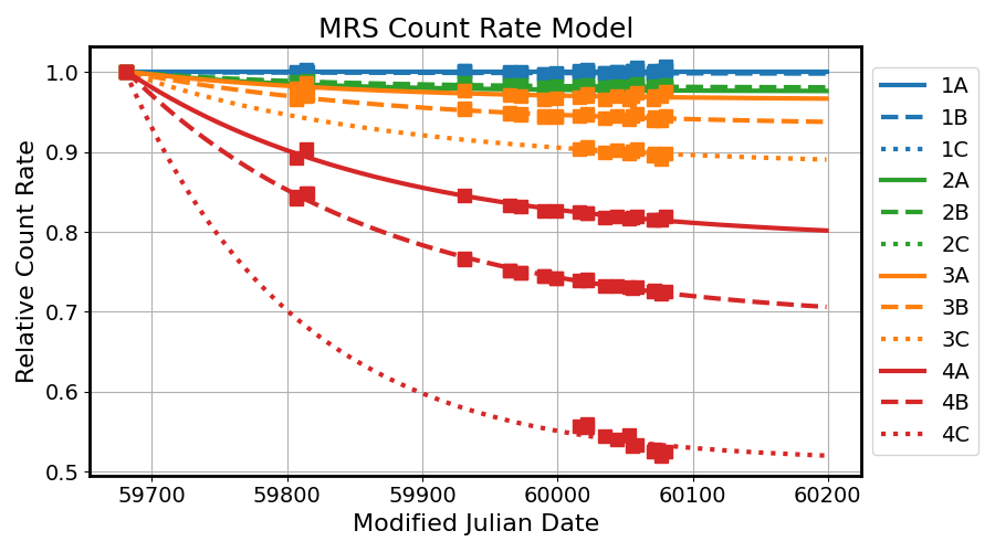
Figure 1: Time-dependent decrease in the observed MRS count rate as measured from internal calibration lamp exposures. Points illustrate measurements at the central wavelength of each of the 12 MRS bands; curves represent the best fit models used for correction in the pipeline. See JDox for an updated version of this figure.
The MRS PHOTOM Reference File contains a table of correction coefficients
for each band in which a correction has been determined. If the time-dependent
coefficients are present in the reference file for a given band, the photom step will
apply the correction to the exposure being processed.
Time-Dependent Corrections
For any mode other than MIRI MRS, the reference file can optionally contain tables of coefficients that are used to apply time-dependent corrections to the scalar conversion factor, based on the observation date of the exposure being processed. Each table present describes a different functional form for the time-dependent sensitivity loss: exponential, linear, or power-law. If multiple tables are present, the corrections are multiplied together before being applied. If no tables are present, no time correction is applied. These coefficient tables also contain the descriptive exposure parameters present in the photometric data table (e.g., filter, pupil, grating), and the rows present must match the length and order of the photometric table.
The correction factor described in all cases is defined as the fractional amount of light recorded now divided by the light recorded on the zero-day MJD (t0). The scalar conversion factor is divided by the correction factor to account for the sensitivity loss.
For a linear correction, the correction factor (corr) is defined as:
where lossperyear (fractional loss of throughput per year, e.g., 0.1 is 10% in 1 year) and t0 (reference day in MJD) are stored as coefficients in the TIMECOEFF_LINEAR extension of the PHOTOM Reference File.
For an exponential correction:
where amplitude, t0 (reference day in MJD), tau (e-folding time constant), and const (long-term asymptote) are stored as coefficients in the TIMECOEFF_EXPONENTIAL extension.
For a power law correction:
where year1value (relative throughput one year after t0), t0 (reference day in MJD), tsoft (softening parameter for the initial decline), and alpha (loss coefficient) are stored as coefficients in the TIMECOEFF_POWERLAW extension.